Non-negative matrix factorization
Reference: Non-negative matrix factorization
NMF is an alternative approach to decomposition that assumes that the data and the components are non-negative. NMF can be plugged in instead of PCA or its variants, in the cases where the data matrix does not contain negative values. It finds a decomposition of samples X into two matrices W and H of non-negative elements, by optimizing for the squared Frobenius norm:
This norm is an obvious extension of the Euclidean norm to matrices. (Other optimization objectives have been suggested in the NMF literature, in particular Kullback-Leibler divergence, but these are not currently implemented.)
Using: sklearn.decomposition.NMF
[1]:
%matplotlib inline
%load_ext autoreload
%autoreload 2
import os, sys
import numpy as np
from skimage import io
import matplotlib.pylab as plt
sys.path += [os.path.abspath('.'), os.path.abspath('..')]  # Add path to root
import notebooks.notebook_utils as uts
:0: FutureWarning: IPython widgets are experimental and may change in the future.
load datset
[2]:
p_dataset = os.path.join(uts.DEFAULT_PATH, uts.SYNTH_DATASETS_FUZZY[0])
print ('loading dataset: ({}) exists -> {}'.format(os.path.exists(p_dataset), p_dataset))
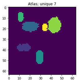
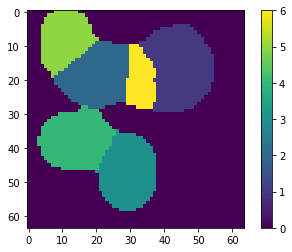
p_atlas = os.path.join(uts.DEFAULT_PATH, 'dictionary/atlas.png')
atlas_gt = io.imread(p_atlas)
nb_patterns = len(np.unique(atlas_gt))
print ('loading ({}) <- {}'.format(os.path.exists(p_atlas), p_atlas))
plt.imshow(atlas_gt, interpolation='nearest')
_ = plt.title('Atlas; unique %i' % nb_patterns)
loading dataset: (True) exists -> /mnt/30C0201EC01FE8BC/TEMP/atomicPatternDictionary_v0/datasetFuzzy_raw
loading (True) <- /mnt/30C0201EC01FE8BC/TEMP/atomicPatternDictionary_v0/dictionary/atlas.png
[3]:
list_imgs = uts.load_dataset(p_dataset)
print ('loaded # images: ', len(list_imgs))
img_shape = list_imgs[0].shape
print ('image shape:', img_shape)
loaded # images:  800
image shape: (64, 64)
Pre-Processing
[5]:
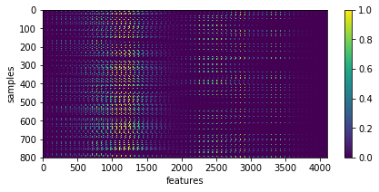
X = np.array([im.ravel() for im in list_imgs])  # - 0.5
print ('input data shape:', X.shape)

plt.figure(figsize=(7, 3))
_= plt.imshow(X, aspect='auto'), plt.xlabel('features'), plt.ylabel('samples'), plt.colorbar()
input data shape: (800, 4096)
[6]:
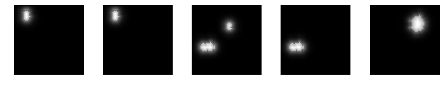
uts.show_sample_data_as_imgs(X, img_shape, nb_rows=1, nb_cols=5)
Non-negative matrix factorization
[7]:
from sklearn.decomposition import NMF
nmf = NMF(n_components=nb_patterns, max_iter=99)

X_new = nmf.fit_transform(X[:1200,:])
print ('fitting parameters:', nmf.get_params())
print ('number of iteration:', nmf.n_iter_)
fitting parameters: {'beta_loss': 'frobenius', 'shuffle': False, 'verbose': 0, 'solver': 'cd', 'l1_ratio': 0.0, 'max_iter': 99, 'init': None, 'random_state': None, 'n_components': 7, 'tol': 0.0001, 'alpha': 0.0}
number of iteration: 98
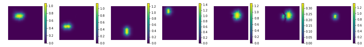
show the estimated components - dictionary
[8]:
comp = nmf.components_
coefs = np.sum(np.abs(X_new), axis=0)
print ('estimated component matrix:', comp.shape)

compSorted = [c[0] for c in sorted(zip(comp, coefs), key=lambda x: x[1], reverse=True) ]
uts.show_sample_data_as_imgs(np.array(compSorted), img_shape, nb_cols=nb_patterns, bool_clr=True)
estimated component matrix: (7, 4096)
[9]:
ptn_used = np.sum(np.abs(X_new), axis=0) > 0
atlas_ptns = comp[ptn_used, :].reshape((-1, ) + list_imgs[0].shape)

atlas_ptns = comp.reshape((-1, ) + list_imgs[0].shape)
atlas_estim = np.argmax(atlas_ptns, axis=0) + 1
atlas_sum = np.sum(np.abs(atlas_ptns), axis=0)
atlas_estim[atlas_sum < 1e-1] = 0
_ = plt.imshow(atlas_estim, interpolation='nearest'), plt.colorbar()
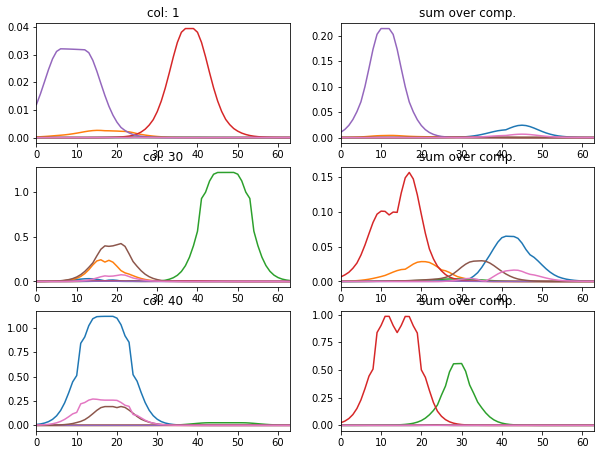
[12]:
l_idx = [1, 30, 40]
fig, axr = plt.subplots(len(l_idx), 2, figsize=(10, 2.5 * len(l_idx)))
for i, idx in enumerate(l_idx):
    axr[i, 0].plot(atlas_ptns[:,:,idx].T), axr[i, 0].set_xlim([0, 63])
    axr[i, 0].set_title('col: {}'.format(idx))
    axr[i, 1].plot(np.abs(atlas_ptns[:,idx,:].T)), axr[i, 1].set_xlim([0, 63])
    axr[i, 1].set_title('sum over comp.')
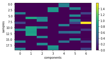
particular coding of each sample
[16]:
plt.figure(figsize=(6, 3))
plt.imshow(X_new[:20,:], interpolation='nearest', aspect='auto'), plt.colorbar()
_= plt.xlabel('components'), plt.ylabel('samples')

coefs = np.sum(np.abs(X_new), axis=0)
# print 'used coeficients:', coefs.tolist()
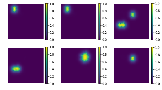
backword reconstruction from encoding and dictionary
[17]:
res = np.dot(X_new, comp)
print ('model applies by reverting the unmixing', res.shape)
model applies by reverting the unmixing (200, 4096)
[20]:
uts.show_sample_data_as_imgs(res, img_shape, nb_rows=2, nb_cols=3, bool_clr=True)
[ ]: